Why do Prices Change? Supply, Demand and the Fulton Fish Market
Why can fish prices rise sharply from one morning to the next, even though the fish itself has not changed? Fishermen bring in different amounts of fish every morning, partly depending on the weather. [1] However, demand for fish from consumers and restaurants often does not change based on the weather. This causes consumers to compete with one another for the limited supply of fish. It is important to emphasise that the price of the fish doesn’t depend only on the size of the catch; it also depends on how supply compares with consumers’ demand. How do these forces interact to produce a market price?
What is Supply and Demand?
Demand is the relationship between the price of a product, and the quantity consumers are willing and able to buy. Here, the words “willing and able” are important as a consumer who only “wants” a product will not necessarily have effective demand if they are unable to afford it.
Supply is the relationship between the price of the product, and the quantity producers are willing and able to offer for sale at different prices. “Willing and able” are important because a seller may have the capacity or stock to supply a product but may not find it worthwhile to offer the same quantity at every price. Generally, a higher price gives producers a greater incentive to supply more.
The Law of Demand
The law of demand states that there is an inverse relationship between price and quantity demanded, assuming all other variables that affect demand remain constant. This means that a rise in price will usually decrease the quantity demanded. This may be because consumers can no longer afford the product or may switch to cheaper alternatives. As a result, the fall in sales volume may offset some or all of the additional revenue gained from the higher price.
For instance, if the price of whiting (a type of fish) increases, restaurants and consumers may order less or substitute it for other foods.
Point of clarification:
“Quantity demanded” and “demand” are not the same thing. “Quantity demanded” is one specific amount that customers are willing and able to buy at a specific price. For instance, the quantity demanded is 5,427 pounds of whiting when the price per pound is $1 per pound. By contrast, “demand” is the relationship between a range of prices and the corresponding quantities demanded; including how much customers would buy at every other possible price.
Example:
Suppose a concert ticket costs £50 and 1,200 people want one
Quantity demanded: 1,200 tickets at £50 each
Demand:
At £30, 2,000 people would buy the ticket
At £50, 1,200 people would buy the ticket
At £80, 500 people would buy the ticket
The simplest way to understand this is that a price change causes a change in quantity demanded. On the other hand, a non-price change (e.g. income, population, tastes, expectations or the price of substitutes) causes a change in demand.
Using this distinction prevents us from confusing movement along the demand curve with shifts of the demand curve. Only a change in price causes movement along the demand curve; changes in income, tastes, expectations or the prices of related goods shift the entire curve.
Imagine you want to know how people dress at different temperatures. You choose 5℃, 15℃ and 25℃, then record how many people wear coats. More people wearing coats does not make the temperature fall. Instead, the temperature determines how many people wear coats.
Likewise, on a demand curve, price determines quantity demanded. We are observing how consumers respond to different prices, not how different quantities create prices.
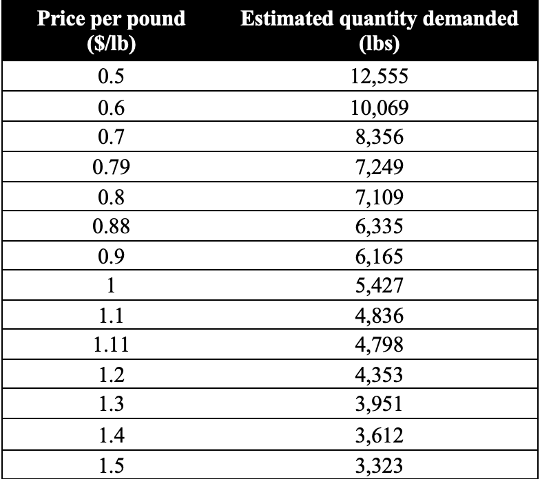
Table 1: Price and Quantity Demanded of Whiting at the Fulton Fish Market
This demand schedule is a calibrated estimate based on data collected over 111 days between late 1991 and early 1992 by researchers from the University of Oxford Department of Economics. [2] Although the data are quite old, the modern demand law (refined in 1890 by Alfred Marshall) still reliably depicts human behaviour. Governments, businesses and everyday markets still use this model to understand how consumers respond to changing prices. The points are plotted on the graph to represent the demand curve illustrated below.
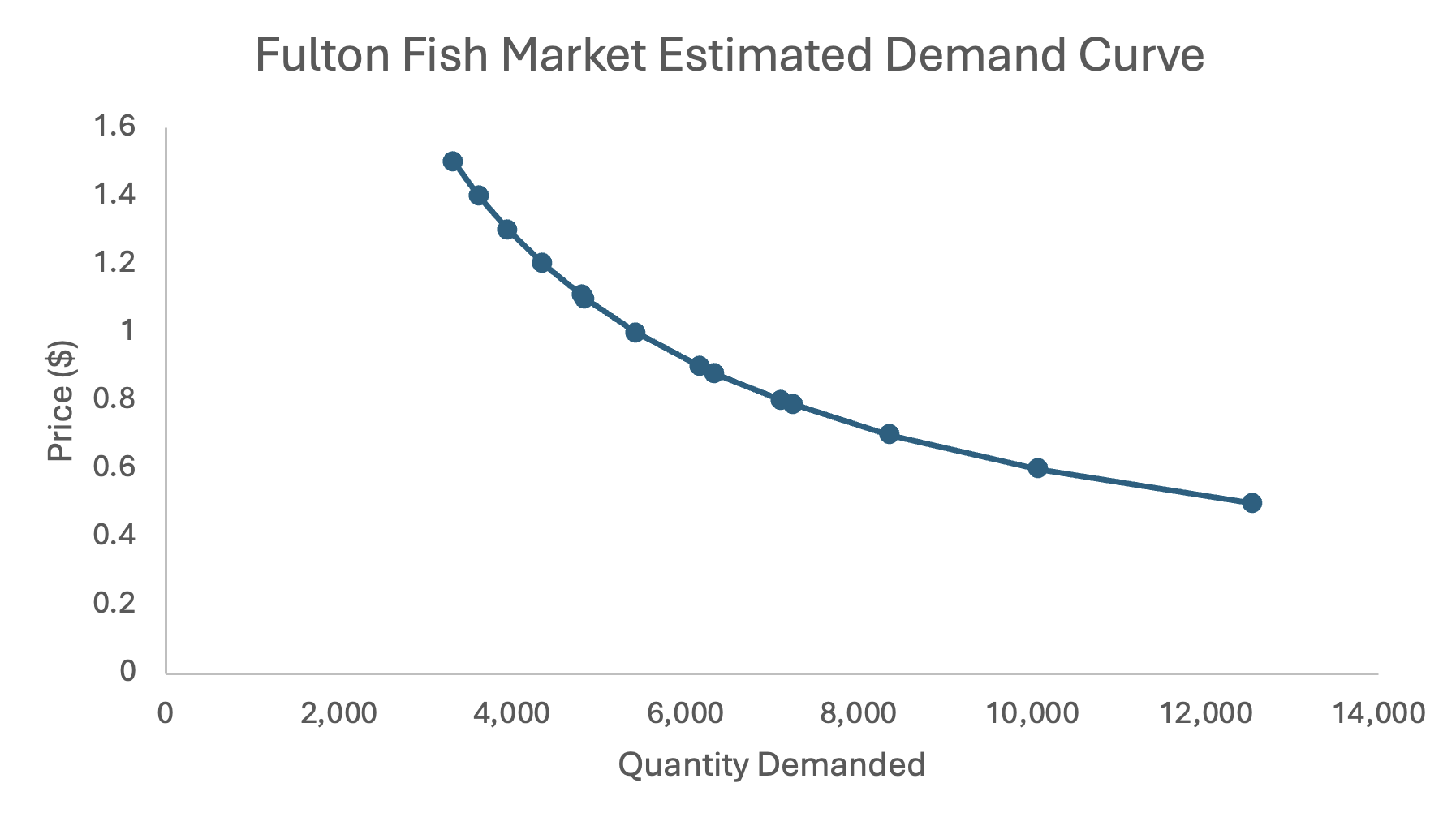
Figure 1: Calibrated demand schedule and demand curve for whiting
This demand schedule shows how much whiting consumers are willing to buy at each price while holding other influences constant. Its negative gradient supports the law of demand; when price increases, quantity demanded decreases, following the inverse relationship.
It is important to note that the demand schedule and curve are both rough estimates as the Oxford report did not provide a neat schedule between price and quantity demanded. Data recorded on different days represent different market outcomes because supply, demand and inventory conditions may all have changed. As we mentioned earlier, the demand law only works along a given demand curve when other factors are held constant; a change in any other variable (income, tax, consumer likes etc.) will shift the entire demand curve, meaning that we cannot simply draw a line through daily sales figures.
Therefore, we can estimate what the demand curve would look like using the data we already have. [3]
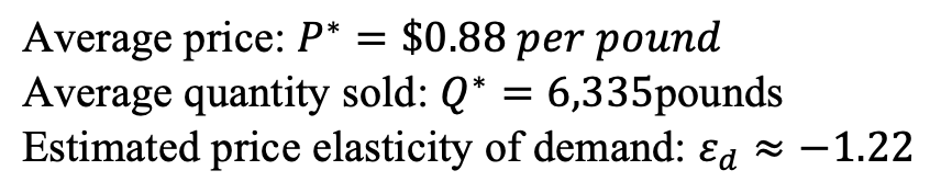
The price elasticity of demand at -1.22 is relatively close to the unit elasticity (which is -1.0) meaning quantity demanded changes by a slightly greater percentage than price.
For example, if a company raises its prices by 1%, sales volume is estimated to fall by approximately 1.22%. Because quantity falls proportionally more than price rises, demand is elastic around this point and total revenue would fall slightly.
To calibrate the demand curve used in Table 1, the average market price and quantity are combined with the estimated elasticity of -1.22. The curve is therefore an illustrative representation of the study’s demand estimate rather than an equation directly published in the report. [4]
Giving the calibrated curve:

We can derive the demand schedule and curve by plugging different prices into the calibrated demand equation.
The Law of Supply
If we think about demand showing us how consumers react to price, supply shows how producers and sellers respond to price.
Quantity supplied is the amount of a good or service a producer is willing and able to produce and sell on the market at each price. Assuming other factors remain constant, a higher price generally gives producers a greater incentive to supply more. For instance, when bread prices rise, bakers may bake additional batches, schedule more workers, or lengthen their opening hours to make more revenue. This means that a higher price can directly increase quantity supplied within the same day or week, producing a more standard, upward-sloping supply curve.
Unlike a bakery, when whiting prices rise, fishermen cannot change the previous night’s catch after seeing the morning price. [5] Dealers can respond to price only to a limited extent through inventory decisions. [6]
This in turn produces an illustrated vertical supply curve, which means the same quantity of whiting is available regardless of the current market price in the very short run.
We display two supply schedules to differentiate between clear weather supply and stormy weather supply. [7]
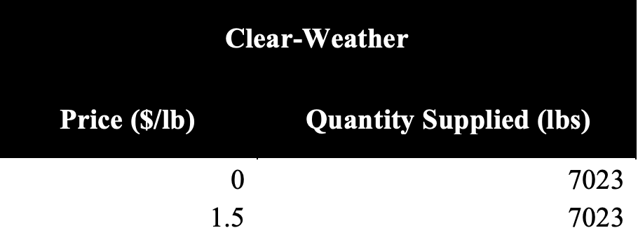
Table 2a: Clear Weather Illustrative Short-run Supply Schedule
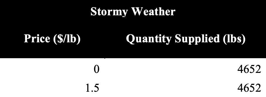
Table 2b: Stormy Weather Illustrative Short-run Supply Schedule
Below are the illustrative supply curves for both types of offshore weather. The vertical supply lines represent perfectly inelastic supply in our simplified model, because the catch of whiting cannot change once the fish have arrived at the market. [8] For example, if 7,000 lbs of whiting arrive on a clear-weather day; whether the price is $1.50 /lb or $0.60/lb or $0.40/lb, the supply of Whiting remains at 7000 lbs.
Although whiting remained saleable for up to four days, it was usually sold on the day it arrived or the following day. [9] Inventory therefore made actual supply slightly more flexible than the vertical curves suggest, but short-run supply remained relatively inelastic.
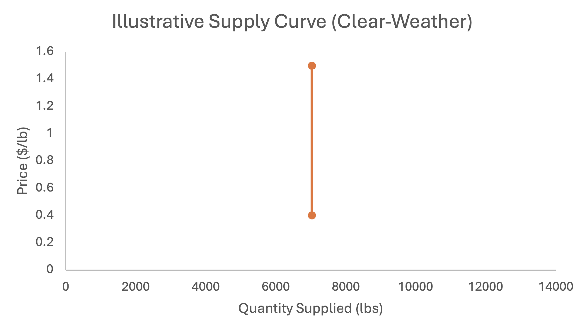
Figure 2: Illustrative short-run supply curve (Clear-Weather)
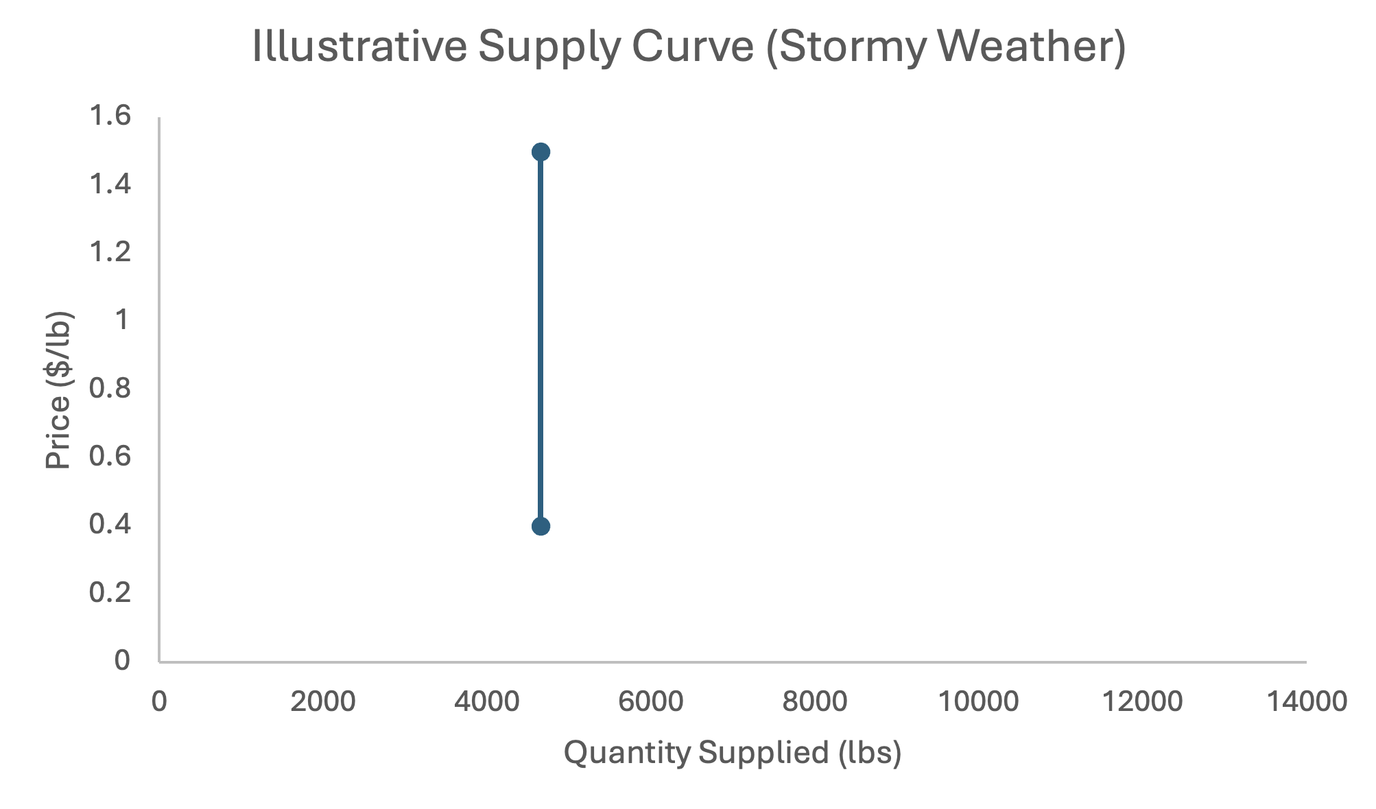
Figure 3: Illustrative short-run supply curve (Stormy-Weather)
Point of Clarification
Similar to demand and quantity demanded, supply and quantity supplied differ in the same way. A change in price causes a movement in quantity supplied, while other factors, such as weather shift the entire supply curve.
Market Equilibrium
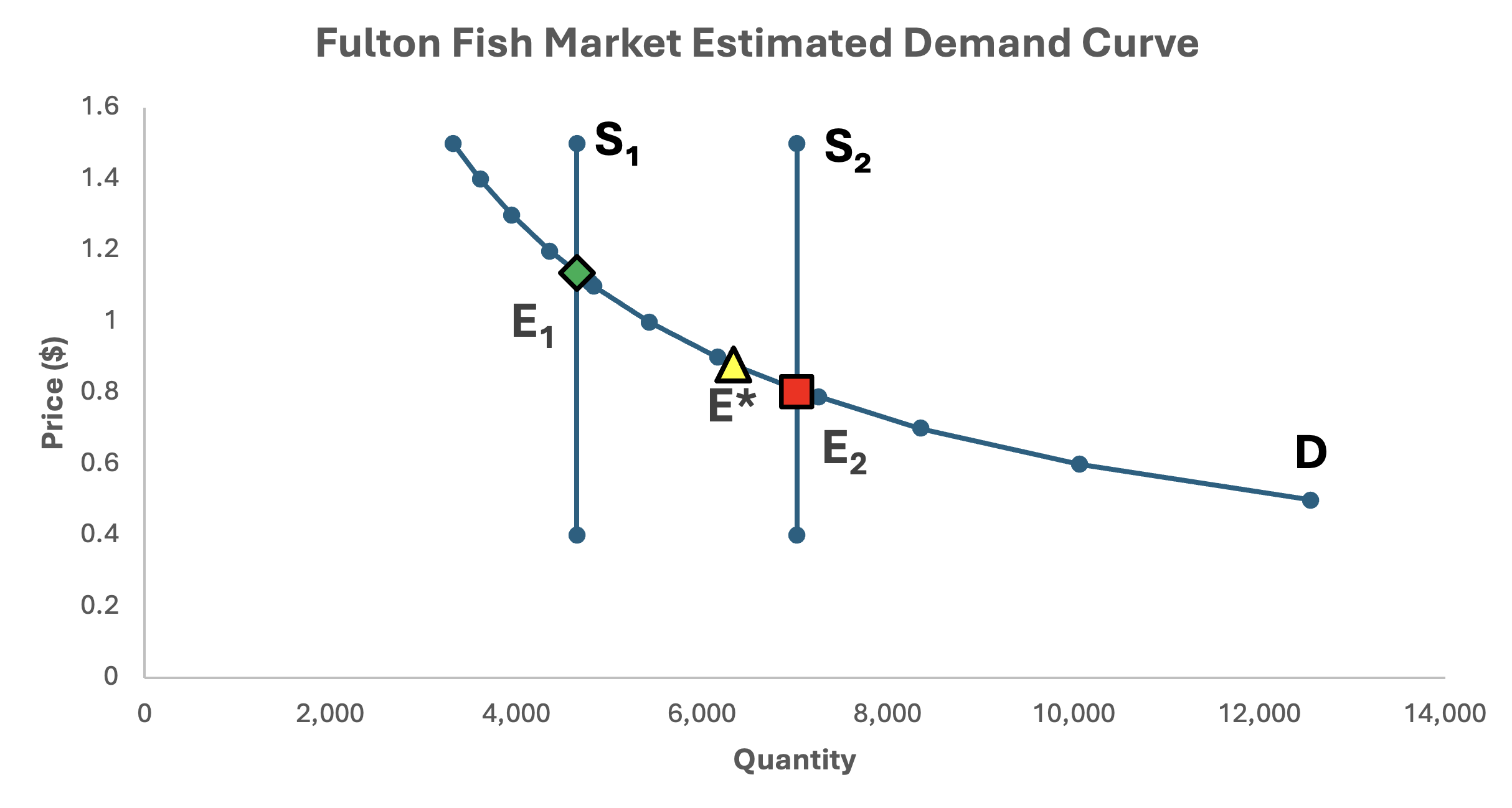
Figure 4: Calibrated equilibrium in the Fulton Fish Market
Note:
S1: Supply Curve (Stormy Weather)
S2: Supply Curve (Clear Weather)
D: Demand Curve
E*: Average equilibrium price
E1: Stormy Weather Equilibrium Price
E2: Clear Weather Equilibrium Price
This is a calibrated representation of average market outcomes, not proof that every trading day cleared at exactly these equilibrium points. [10]
The equilibrium price can be quickly calculated solving the supply and demand relationships for the same market. The point at which these curves intersect is called the equilibrium price. In Figure 4, E1 represents the stormy-weather equilibrium and E2 represents the clear-weather equilibrium. This is the only point where the plans of consumers and sellers agree: quantity demanded equals quantity supplied.
The equilibrium point is where there is neither a shortage nor a surplus, so there is no immediate pressure for price to change.
Equilibrium price: the price where quantity demanded and quantity supplied are equivalent
Equilibrium quantity: the amount traded at the equilibrium price
After combining the three curves we can derive an average market outcome: [11]

Shortage
When the market is not at an equilibrium price, economic pressure will push the market to move toward the equilibrium price and equilibrium quantity.
For example, a stormy day may cause the quantity supplied of whiting to drop from 7023 lbs to 4652 lbs. [12] The vertical supply curve will shift from S2 to S1, moving to the left.
However, at the original E2 price of about $0.80, the quantity demanded is approximately 7023 lbs, which now exceeds the fixed quantity supplied of 4,652 lbs. Whiting sells quickly as consumers rush to buy more at the low price, and some consumers are unable to obtain the amount they want.
Sellers now realise that the existing price is too low to clear the market, so the market price rises to maximise revenue. The price continues to increase until the new quantity demanded equals the fixed quantity supplied. This shifts the price back to the new stormy-weather equilibrium, E1.
Surplus
By contrast, when the market price is above the equilibrium price, the quantity demanded, found on curve D, is lower than the fixed quantity supplied. This causes some fish to remain unsold. Because whiting is perishable, sellers have an incentive to reduce the price.
The new, lower price causes quantity demanded to rise again, and the price continues to fall until the quantity demanded equals to the quantity supplied. The market is brought back to equilibrium.
To summarise, when the price drops below the equilibrium price there is a shortage, while a surplus occurs when the price rises above the equilibrium price.
Point of Clarification
If the equilibrium price is so ideal, why does the price change anyway? The price may not remain at the same equilibrium because the equilibrium point itself changes when supply or demand changes.
Suppose clear weather produces a supply of 7,023 pounds. The clear-weather supply curve intersects demand at , giving a price of about $0.80.
After stormy weather, only 4,652 pounds arrive. Supply shifts left. The old point is no longer an equilibrium because that quantity of fish is not available. The price therefore moves towards the new stormy-weather equilibrium, E1, as supply decreases.
Price only remains at the same equilibrium when the conditions determining supply and demand remain unchanged. When either one of these changes, the equilibrium point will shift, causing the market price to shift towards the new equilibrium.
Demand can also change equilibrium
Demand can also shift the equilibrium point. Changes in income, tastes, population, expectations, and prices of substitutes can also create a shortage or surplus at the previous price. For instance, if more restaurants begin serving whiting, demand shifts right. At the old price, buyers want more fish than is available, creating a shortage. Price rises until a new equilibrium is reached.
Conclusion
The Fulton Fish Market shows how prices can adjust when supply or demand changes unexpectedly. Prices are determined through the interaction of changing supply and demand curves, which produce an equilibrium based on the conditions at a particular time. The Fulton Fish Market provides a clear example: weather changed the quantity of fish available, and price adjusted to match this changing supply with buyers’ demand.
The laws of demand and supply also operate in markets ranging from ride-hailing services such as Uber to electricity during peak periods. In each case, price acts as a signal that helps balance limited supply with changing demand.
Footnotes
[1] Kathryn Graddy, “Markets: The Fulton Fish Market,” University of Oxford Department of Economics Discussion Paper No. 254, January 2006. Graddy explains that offshore weather conditions affected the quantity of whiting caught and that stormy weather reduced quantities supplied while increasing prices.
[2] Graddy, “Markets: The Fulton Fish Market.” The dataset contains 111 trading-day observations from late 1991 and early 1992. The paper reports an average price of approximately $0.88 per pound and an average daily quantity of 6,335 pounds. The demand schedule shown in this article is a calibrated estimate rather than a schedule directly published in the paper.
[3] Graddy, “Markets: The Fulton Fish Market.” The study reports an instrumental-variable estimate of the price elasticity of demand of approximately −1.22 when weekday and weather controls are included.
[4] The linear demand equation Qd=14,063−8,782P is a calibration used for this article rather than an equation directly published by Graddy. It is derived from the reported average price of $0.88 per pound, average quantity of 6,335 pounds and elasticity estimate of approximately −1.22.
[5] Kathryn Graddy and Peter E. Kennedy, “When Are Supply and Demand Determined Recursively Rather Than Simultaneously? Another Look at the Fulton Fish Market Data,” University of Oxford Department of Economics Discussion Paper No. 297, December 2006. The authors explain that the day’s potential supply was largely determined by the previous night’s catch, although current prices could still affect the quantity offered through inventory decisions.
[6] Graddy and Kennedy, “When Are Supply and Demand Determined Recursively Rather Than Simultaneously?” Dealers could add to or draw down inventories, meaning that effective daily supply was not literally fixed and could respond to current prices.
[7] The illustrative clear-weather and stormy-weather quantities of 7,023 pounds and 4,652 pounds are calibrated values used in this article and are not figures directly reported by Graddy. The underlying empirical result is that, holding day of the week constant, average quantity on clear-weather days was 2,371 pounds higher than on stormy-weather days.
[8] The vertical supply curves are simplified short-run representations used for explanation. Graddy notes that the day’s whiting had been delivered before the market opened, but dealers could still trade between themselves and carry inventories across days. The original research therefore does not estimate a literally vertical empirical supply curve.
[9] Graddy, “Markets: The Fulton Fish Market.” Whiting could remain sufficiently fresh to sell for up to four days, but it was usually sold on the day it was received or the following day.
[10] Figure 4 combines the calibrated demand curve used in this article with the illustrative clear-weather and stormy-weather supply curves. The equilibrium points shown are therefore constructed for explanation and are not individual daily equilibria directly reported in the Fulton Fish Market dataset.
[11] Graddy reports an average observed price of approximately $0.88 per pound and an average daily quantity of 6,335 pounds across the sample. These values are sample averages and should not be interpreted as one permanent equilibrium price and quantity.
[12] The shortage example uses the article’s illustrative quantities of 7,023 and 4,652 pounds. The empirical evidence behind the example is Graddy’s finding that clear-weather quantity was on average 2,371 pounds higher than stormy-weather quantity, while clear-weather prices were on average $0.32 per pound lower.
